Chapter 7: Steps for Multivariate Analysis and Results
This chapter reviews two Basic multivariate analyses: 1) Multiple Linear Regression and 2) Multiple Logistic Regression. Two multivariate analyses are widely used to examine when there are two or more independent variables (also called the predictor variables) on which the dependent variable (also called the outcome variable) is assumed to relate. Multivariate analyses aim to examine whether each independent variable predicts the dependent variable when all other independent variables are controlled for. Two multivariate analyses also examine the strengths of the relationship of IV on DV. Two multivariate analyses are chosen based on the level of measurement of the dependent variable. Thus, when there are two or more independent variables and the DV is an interval or ratio level variable as a scale level in SPSS, we choose a multiple linear regression analysis. When the DV is a binary nominal measure, we use multiple logistic regression.
Multiple Linear Regression
Multiple linear regression assumes that each IV has a linear relationship with the DV. Since it includes multiple IVs to predict the DV, there are some preliminary tests required among multiple IVs such as Homoskedsticity[1], no autocorrelation[2], normal distribution, and multicollinearity[3]. This chapter assumes those assumptions are met to review the next steps.
Other than those assumptions, conducting a multiple regression analysis requires that all IVs in the study are scale measures (interval/ratio level of measures). What it means is that IVs of nominal and ordinal measures are required to be converted into scale measures. This is a bit confusing concept for students in terms of how to change the nominal and ordinal measures to scale measures. Binary/Dichotomous nominal variables are relatively easy to convert into scale measures since we can assign values to be 0 and 1 numeric values (yes=1, no=0), which are called “Dummy Variables.” We can assume dummy variables are scale measures since they have only 0 and 1 numeric values and we can treat them as scale measures. In case we assign values 1 for females and 2 for males in the original dataset, we can recode it into a new gender variable to have 1 for females and 0 for males or 1 for males and 0 for females.
Dummy variables are a set of binary/dichotomous numeric variables that represent categorical variables that have only two groups such as gender, or yes/no. As a general rule, a new dummy variable is coded 1 if a certain trait is present like Yes, or 0 if absent like No. When we code a group as 0, we call this group as the reference group for the test. In this gender example, males are assigned to be 0 as the reference group or vice versa. The reference group is the base group to be compared with other groups as females will be compared to males in the SPSS output when we interpret the results.
From a binary nominal measure of gender, we recode and recreate only one variable although the variable has two groups of females and males. This indicates that the number of dummy variables that should be created can be obtained by subtracting the number 1 from the number of groups of the variable. For example, for the gender variable with two groups, one dummy variable needs to be created by subtracting the number 1 from 2 (2-1=1).
Table 7-1. The Number of Dummy Variables to be Created | |
Old Variable | New Dummy Variables |
Gender
| One new variable (2-1=1) Female: 1. Yes, Female 0. No Female Reference group |
Race
| Four new variables (5-1=4) Asian: 1. Yes, Asian 0. No Asian Black: 1. Yes, Black 0. No Black Latino: 1. Yes, Latino 0. No Latino Reference Group Other: 1. Yes, Other 0. No Other |
Housing
| Three new variables (4-1=3) Reference group Rent: 1. Yes, rent 0. Not own Co-housed: 1. Yes, co-housed 0. Not co-housed No-housing: 1. Yes no housing 0. Not no-housing |

Figure 7-1. Steps to Create Dummy Variables
In case the variable has five groups as presented in Table 7-1, we need to create four dummy variables (5-1=4). The race/ethnicity variable has five groups with Asian, Black, Latino, White, and Other. Then we select one group to be the reference group and create four dummy variables. In general, the Whites group is chosen for the reference group, and we create the four variables of Asian, Black, Latino, and Other by assigning 1 for Asian, Black, Latino, and Other and 0 for all other racial/ethnic groups and creating four dummy variables. Figure 7-1 presents steps to create dummy variables by using recoding process in “Transform” and “Recode into Different Variable,”[4] as learned in Chapter 5.
Once we confirm all IVs and DV are scale measures by creating dummy variables from nominal independent variables, we can conduct multiple regression analysis. Table 7-2 and Figure 7-2 present steps to conduct multiple regression.

Figure 7-2 Steps of Multiple Linear Regression

Figure 7-3 SPSS Outputs of Multiple Linear Regression
Table 7-2. Steps for Multiple Linear Regression |
1. Click ‘Analyze’ on the top menu in Data View or in Variable View 2. Click ‘Regression’ from the options in about the middle 3. Choose ‘Linear’ on the second option 4. Choose a dependent variable from the variable list on the left from the pop-up box 5. Click the arrow or double-click the variable to move DV to “Dependent:” on the right side 6. Choose all independent variables and move them to “Independent(s):” from demographic variables first to primary IVs 7. Click “Statistics” on the top blue button 8. Click “Estimates” “Model fit” and “Descriptives” 9. Click “Continue” 10. Click ‘OK’ |
Figure 7-3 displays an example of multiple regression that examines whether bullying victimization predicts suicidal ideation along with demographic variables of age, gender, and race. The first table “Model Summary” provides information on whether this model with bullying and demographic variables explains suicidal ideation with a value of “Adjusted R Square.” In this example, this model with bullying and demographic variables explains 15% of the variance of the dependent variable of suicidal ideation (0.15x100 = 15%). The second table “ANOVA” provides information about whether this model significantly predicts suicidal ideation with the values of “F” and “Sig.” This example of the model is statistically significant in explaining suicidal ideation at the level of p = 0.05 as F-value is 33.028 with df = 1259 and the p-value is less than 0.001. The third table “Coefficients” provides information about whether each of IVs significantly predicts the DV. In this column, we check the “Sig” in the last column about whether any of the p-values for IVs are smaller than 0.05. In this example, female dummy, Asian dummy, and bullying victimization significantly predict suicidal ideation. An example of a write-up and table presentation for the Results section are shown in Tables 7-3 and 7-4.
Table 7-3. Sample Write-up of Multiple Linear Regression Results |
Multiple regression was conducted to examine whether the study model of bullying and demographic variables explains suicidal ideation. Results showed that this study model was statistically significant (F = 33.028, df = 1,259, p < 0.001). The full model explained 15% of the variance of suicidal ideation. An examination of individual independent variables showed that being a female (β = .177, t = 6.777, p < .001), being an Asian (β = .085, t = 3.191, p = .001), and bullying victimization (β = .325, t = 12.245, p < .001) significantly predict suicidal ideation after controlling for other independent variables while age (p = .160), being a Black (p = .608), being a Hispanic (p = .405), and being other racial groups (p = .551), were not significantly related to suicidal ideation. |
Table 7-4. Table Template of Multiple Linear Regression Results | ||||
Table # Results from Multiple Regression for Suicidal Ideation and Bullying | ||||
B | β | p | ||
Constant | .188 | .108 | ||
Age | .030 | .037 | .160 | |
Gender | .359 | .177 | .001 | |
Whites (reference group) | ||||
Asian | .389 | .085 | .001 | |
Black | .041 | .014 | .608 | |
Hispanic | .080 | .022 | .405 | |
Other | .041 | .016 | .551 | |
Bullying Victimization | .519 | .325 | .001 | |
F = 33.028, df = 1,266, p < .001, R2 = .15 | ||||
Multiple Logistic Regression
Multiple Logistic Regression is used to examine whether multiple independent variables in the study predict a binary/dichotomous dependent variable, which is a nominal measure like a dummy variable with Yes =1 and No=0. Table 7-5 and Figure 7-4 present steps to conduct a multiple logistic regression analysis.
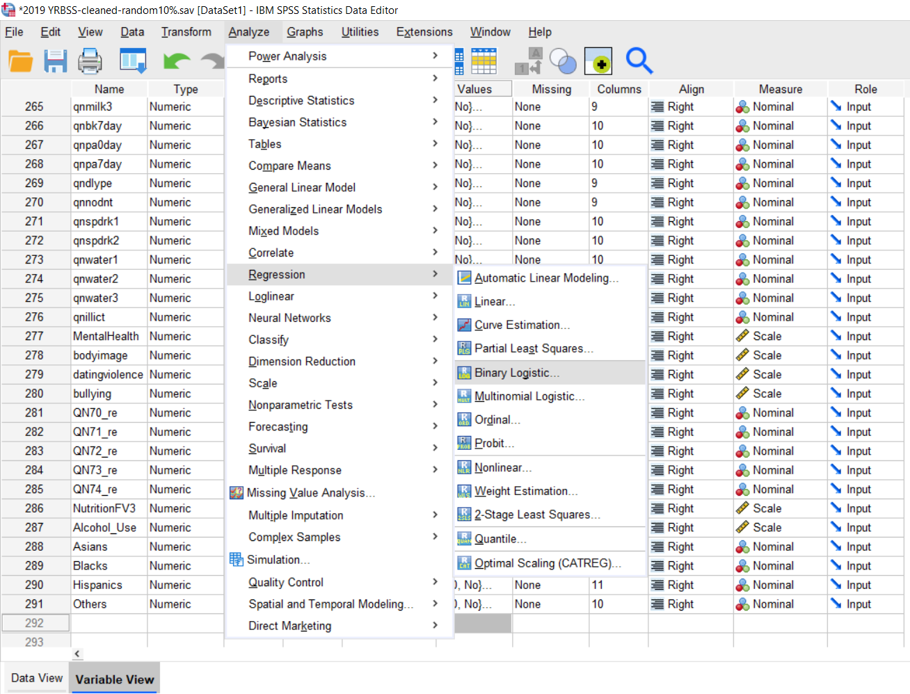

Figure 7-4. Steps of Multiple Logistic Regression
Table 7-5. Steps for Multiple Logistic Regression |
1. Go to ‘Analyze’ on the top menu in Data View or in Variable View 2. Choose ‘Regression’ from the options in about the middle 3. Choose ‘Binary Logistic Regression’ on the fifth option 4. Choose a binary dependent variable from the variable list on the left from the pop-up box 5. Click the arrow or double-click the variable to move DV to “Dependent:” on the right side 6. Choose all independent variables and move them to “Covariates:” from demographic variables first to primary IVs 7. Click “Options” on the third blue button 8. Choose “CI for exp(B)” on the pop-up box 9. Click “Continue” 10. Click ‘OK’ |
Figure 7-5 displays SPSS outputs of multiple logistic regression analysis. In Figure 7-5, the first table “Omnibus Tests of Model Coefficients” provides information about whether the study model is statistically significant to explain the study DV. In this example, the model significantly explains depression as feeling sad and hopeless at the level of p = 0.05 as “Sig.” is less than 0.001 with Chi-square value = 159.274 and df = 7. The second table “Model Summary” shows that the degree of the model explains the DV. In this table, using the value of “Nagelkerke R Square,” this study model of bullying and demographic variables explains 16.1% of the variance of the dependent variable of depression, feeling sad and hopeless. The fourth table “Classification Table” provides information on how many cases can be explained by the study model. In this example, overall 68.7% of the cases were classified with the model. The last table “Variables in the Equation” provides information about whether each of the independent variables significantly predicts the dependent variable. We review the values of “Sig.” for each variable and use values of ‘B’, ’Sig.’, ‘Exp (B)’, and ‘95% CI for Exp(B)’ with Lower and Upper values for each variable. In this example, age, females and bullying victimization significantly predict depression.
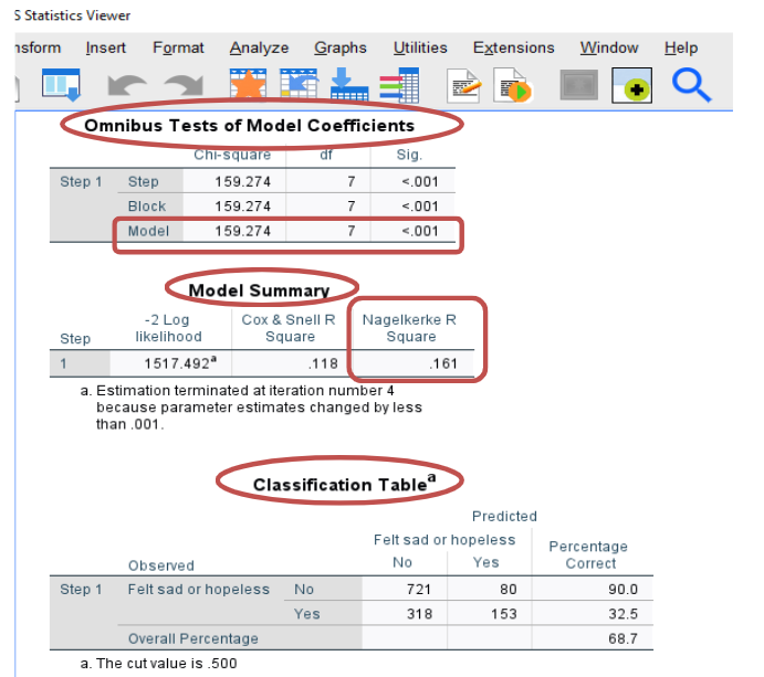

Figure 7-5 SPSS outputs of Logistic Regression
Sample write-up and table presentation for the Results section are as follows.
Table 7-6. Sample Write-up of Multiple Logistic Regression Results |
A logistic regression was conducted to examine the model to explain depression by age, gender, race, and bullying victimization. The logistic regression model was statistically significant (χ2 (df = 7) = 159.274, p < .001). The model explained 16.1% of the variance in being depressed or not and correctly classified 68.7%. Being older (OR = 1.113, p = .033), being a female (OR = 2.352, p < 0.001), and experiencing bullying victimization (OR = 2.485, p < 0.001) significantly predict depression, indicating being older, being a female, and experiencing bullying victimization increases the likelihood of being depressed. |
Table 7-6. Table Template of Multiple Logistic Regression Results | ||||
Table # Likelihood of Depression among Adolescents (Logistic Regression) | ||||
B | Exp (B) | p | 95% CI of Exp (B) | |
Constant | -1.880 | .153 | .001 | |
Age | .107 | 1.113 | .033 | 1.009 – 1.228 |
Gender | .855 | 2.352 | .001 | 1.839 – 3.008 |
Whites (reference group) | ||||
Asians | .250 | 1.284 | .377 | 0.738 – 2.232 |
Blacks | -.171 | 0.843 | .375 | 0.577 – 1.230 |
Hispanics | .390 | 1.477 | .076 | 0.960 – 2.270 |
Others | .094 | 1.098 | .558 | 0.802 – 1.503 |
Bullying Victimization | .910 | 2.485 | .001 | 2.038 – 3.029 |
Classification = 68.7%, χ2(df = 7) = 159.274, p < .001, Nagelkerke R2 = .161 | ||||
[1] Variance of error term is the same for independent variable.
[2] Error terms of independent variables are uncorrelated, meaning that each observation is independent..
[3] Two or more independent variables are highly correlated, then one or more IVs need to be removed from the test, meaning all independent variables in the study have no correlation.
[4] Review Chapter 5 for creating a new variable with “Transform” and “Recode into Different Variable.”