Chapter 6: Steps for Bivariate Analysis and Results

        Basic data analyses comprise univariate, bivariate, and multivariate analyses. As we learn about univariate analysis in Chapter 5, uni-variate (one variable) analysis means examining each of the variables one by one at a time. For the Results section of the graduate research paper/thesis, the first table presents sample characteristics with outputs from univariate analyses as displayed in Table 5-1 in Chapter 5. The univariate analysis step is critical as it reviews the data as a cleaning process, and describes the sample characteristics with each of the key variables in research.

On the other hand, bi-variate (two variables) analysis means examining two variables at a time. Bivariate analysis is a part of inferential statistics, which examines the association between two variables, in particular, whether the two variables are statistically related and can infer the relationship between the two variables based on probability theory^[1]. Based on bivariate analysis, we can test our study hypotheses developed for the research and presented in Literature Review such as whether the study independent variable (IV) is statistically significantly related to the study dependent variable (DV) in our research with data that we examined.

There is a distinct difference between descriptive and inferential statistics, in other words between univariate and bivariate/multivariate analyses. The scope of univariate analysis is called descriptive statistics and is limited to describing the sample characteristics of a sample. However, bivariate and multivariate analyses are called inferential statistics and aim to make predictions about population beyond the sample and can test hypotheses. Testing hypotheses is the inferential procedure to predict the relationship between IVs and DV from the sample to the population based on statistical tests by calculating the probability that can infer the findings to the population, which determines the significance of the relationship between variables. The significance level which is denoted as Alpha (α) is the probability of rejecting or accepting the study hypotheses. The significance level is usually set either at α = 0.05 (5%) or α = 0.1 (10%). α= 0.05 means that there is a 5% chance of making a conclusion that a relationship exists when there is no actual relationship.

As presented in Table 6-1, there are four major bivariate analyses: 1) Correlation, 2) Independent Sample t-test, 3) Analysis of Variance (ANOVA), and 4) Chi-square test. The first step is to determine which bivariate analytical tool we need to adopt to test the study hypothesis. This decision is based on a combination of the level of measurement of the two variables: 1) Two variables (both IV and DV) are scale measures (interval or ratio), 2) One variable (mainly IV, but can be DV) is nominal/ordinal and the other is scale (mainly DV, but can be IV), and 3) Two variables (both IV and DV) are either nominal or ordinal, definitely not scale measures.

As Table 6-1 presents, the first combination is for Correlation analysis and the third is for Chi-square (χ2) test. The second combination is for Independent Sample t-test and Analysis of Variance (ANOVA). When the IV is a nominal/ordinal measure with only two groups such as gender with females and males or any variables with Yes and No answer categories, we perform an Independent Sample t-test. When the IV is a nominal/ordinal measure with three or more groups such as race/ethnicity, marital status, and occupation with multiple occupational groups, we choose an Analysis of Variance (ANOVA) test. We review four bivariate analyses one by one.

Correlation Analysis

        There are different types of Correlation analysis. The most frequently used correlation analysis is Pearson’s r Correlation, in which the two variables (both IV and DV) are scale measures. Correlation analysis is used to determine whether a relationship between two scale variables is statistically significant or not. The steps for Pearson’s r Correlation in SPSS are presented in Table 6-2 and Figure 6-1.

Figure 6-1. Steps for Pearson’s r Correlation

Figure 6-2. Output from Pearson’s r Correlation Analysis

Once a Pearson r Correlation analysis is conducted, the SPSS output window displays the results as shown in Figure 6-2. The Correlation table is a matrix with two variables in the columns and rows generating four cells. Each cell contains three pieces of information of “Pearson Correlation” in the first line, “Sig. (2-tailed)” in the second line, and “N” in the third line. These pieces of information repeat the next row of another variable.  The value of “Pearson Correlation” is the correlation coefficient indicating a relationship between two variables, “Sig. (2-tailed)” is the probability value of the statistical significance of the relationship between the two variables, “N” is the number of cases included in this analysis. Each cell displays three pieces of information. The first cell in the White part displays the correlation between age and age, which is the correlation between the same variable. Thus, the correlation value is “1,” which means the two variables are identical and show perfect correlation. This is the same in the right cell at the second row because it is the correlation between the same variable of suicidal ideation and the correlation value is “1.”

In this output presented in Figure 6-2, the key concern is the correlation between age and suicidal ideation. The cells of the right on the first row and the left on the second row present the same information because the correlation between age and suicidal ideation is the same as the correlation between suicidal ideation and age regardless of the order of the variables. In this output, the Pearson correlation coefficient is -.012 and we present r = -.012 as a lowercase “r” is a statistical symbol of the Pearson correlation coefficient. This correlation coefficient is not statistically significant with a p-value of .677^[2] at the level of p = 0.05.

In Correlation analysis, the correlation coefficient “r” provides two pieces of information: The direction of the relationship and the Strength of the relationship. The coefficient value is close to “1” (either +1 or -1), indicating a strong correlation between the two variables while the values close to “0” indicate little or no correlation^[3]. The coefficient can be a negative value, which implies two variables have a negative relationship^[4] while a positive value indicates a positive relationship. Based on outputs in Figure 6-2, a sample write-up for the Results is shown in Table 6-3. For the Results section in the graduate research paper, the output can be presented in the form of Table 6-4.  

Independent Sample t-Test        

We conduct an independent sample t-test when the independent variable is a binary nominal variable (two groups of respondents like male/female, yes/no, or experiment/control groups), and the dependent variable is a scale measure (interval or ratio levels). We can also use this test when the IV is a scale measure, and DV is a binary nominal measure. This test is used to compare the means of the scale variable for two groups of the nominal variable. For example, we can compare females’ average income to males’ average income as income is a scale measure while gender is generally made up of two groups of people (females and males). We can also compare the average suicidal ideation level of youth who experienced physical dating violence to the average suicidal ideation level of youth who did not in case suicidal ideation is collected as a scale measure and physical dating violence experience is measured as Yes or No. When we compare the outcomes between experimental and control groups, an Independent Sample t-test can be used.  

Steps to conduct Independent Sample t-test displays in Figure 6-3 and Table 6-5.

Figure 6-3 Steps for Independent t-Test

        Once we conduct the Independent Sample t-test, the SPSS produces Outputs as displayed in Figure 6-4. The Outputs presented in Figure 6-4 are an Independent Sample t-test with gender and suicidal ideation. In Figure 6-4, the first table “Group Statistics” presents the mean scores of two groups of females and males with standard deviation and the number of cases included in the test (N). We compare the mean scores of suicidal ideation between females and males. In this example, the mean score of females is 0.95 while the mean score of males is 0.50, which shows that females’ suicidal ideation is higher than males. However, we are not sure whether this difference is statistically meaningful. The second table “Independent Sample Test” presents the statistical significance. The statistical significance can be checked with “Sig. (2-tailed) with t and df values on the first line. This example of gender differences in suicidal ideation is statistically significant since the p-value is smaller than 0.05 (Sig. (2-tailed) = .000).

Based on the outputs of  Figure 6-4, we can report the test results as follows. Tables 6-6 and 6-7 also show how to present the Independent Sample t-test results in the table format in the Results section.

Figure 6-4 SPSS Outputs of Independent t-Test

One Way Analysis of Variance (ANOVA)

The purpose of One-way ANOVA is the same as Independent Samples t-test as it compares the mean scores of scale variables among 3 or more groups (nominal variable). Thus, one variable is a scale measure (interval/ratio level) (usually the Dependent Variable) and the other variable is a nominal measure with three or more groups (usually the Independent Variable). Theoretically, we assume equal variances of the groups, not mean scores to conduct ANOVA. When the variances among groups are not equal, then we conduct non-parametric tests which means the variables aren’t scale measures. This can be checked with the ANOVA test. Figure 6-5 and Table 6-8 display steps to conduct One-way ANOVA. Figure 6-6 presents SPSS output.

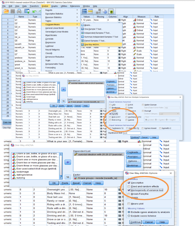
Figure 6-5. Steps for One-way Analysis of Variance

Post Hoc Tests

Figure 6-6. SPSS Outputs of One-way ANOVA

        Figure 6-6 presents SPSS outputs of the One-way ANOVA that examines the school support levels (interval measure) among five race/ethnic groups (nominal measure). The first table “Descriptive” presents mean and standard deviation scores and the number of cases included in ANOVA by five racial/ethnic groups. This table indicates that White youth perceive the highest level of school support, followed by Asian, Other, Black, and Latino youth. The second table of “Test of Homogeneity of Variances” presents whether the variances among five racial groups are equal or not. Since “Sig.” value is 0.000, which is smaller than 0.05, the result indicates that the equal variance of ANOVA assumption is violated.

The third table of “ANOVA” shows whether the differences in school support levels among the five groups are statistically significant or not. We find in the first table that the differences are statistically significant. The “F” value of 19.734 in the second last column and “Sig.” of 0.000 in the last column indicate that the differences in school support levels perceived by the five racial groups are statistically significant. However, we don’t know yet which groups are significantly different because there are five racial groups. The Independent Sample t-test compares two groups, so it is easy to compare which group is higher than the other. ANOVA compares 3 or more groups, so it requires a paired comparison among five groups such as the mean score of Whites’ school support compares to Asians', Blacks', Latinos', and Others’, the mean scores of Asians’ school support compares to Blacks’, Latinos’, Others’, and Whites’, as a total of 20 paired comparison. The fourth table “Post Hoc Multiple Comparison” presents this paired comparison. In this table, we review the fourth column that displays the significance level of a paired comparison. In this example, Asians, Others, and Whites’ school support levels are significantly higher than Latinos.  

        Based on this example, the following is the write-up to report ANOVA results in Tables 6-9 and 6-10.

Chi-Square Test

Chi-Square Test examines an association between the two nominal variables of IV and DV. Table 6-11 and Figure 6-7 present steps for the Chi-Square test. Figure 6-8 presents an example of SPSS outputs. This example is to examine an association between gender and obesity in terms of whether gender is associated with obesity. In this example, IV is gender and DV is obesity.

Figure 6-7. Steps for Chi-Square Test

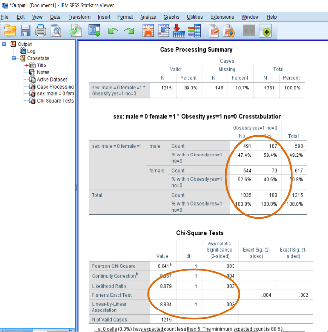
Figure 6-8. SPSS Output of Chi-Square Test

In Figure 6-8, the first table shows the number of cases included in the Chi-Square test. The second table presents two by two cross-tabulation since gender and obesity have two groups. In this table, the column “No, not obese” shows that females are 52.6% (n=544) and males are 47.4% (n=491) while the column “Yes, obese” shows that females are 40.6% (n=76) and males are 59.4% (n=107). This result indicates that more females are not obese in the first column and more males are obese in the second column. This association is statistically significant presented in the third table with the first line of Pearson Chi-Square value =8.841, df=1, and “Asymptotic Significance” =0.003, which is smaller than p=0.05. An example of a write-up for the Chi-Square test results is the following.

Tables 6-12 and 6-13 display how to present the Chi-Square test results in the Results section.