Chapter 5: Data Cleaning and Univariate Analysis Steps in SPSS

        Before we begin a data analysis, we need to review and clean the dataset to prepare for data analysis. This chapter focuses on some useful functions and steps to prepare the dataset for data analysis.

Understanding Variables by the Level of Measurement

        To prepare a dataset for data analysis, we need to check each variable for its accuracy whether there are any errors/typos, how many cases each variable has, and what values the variables have. This helps us find and remove errors and typos in the dataset and decide whether we need to keep the variables as they are or modify them. This step can be done with descriptive statistics.  

        Descriptive statistics are used to understand the sample selected for research purposes by describing the sample characteristics. To understand and describe the sample, we need to review each variable once at a time across all variables, which we call univariate analysis^[1]. To conduct an univariate analysis, it is time to revisit the level of measurement because univariate analyses differ by the level of measurement of the variable. As we already learned in a Research Methods course, there are four levels of measurement; nominal, ordinal, interval, and ratio^[2]. Nominal and ordinal measures do not allow any arithmetic calculations because both measures indicate categories/groups to which research participants belong. Therefore, a numeric value assigned to each variable category (i.e., 1 for female, 2 for male, and 3 for other) has no mathematical quantity. Thus, variables measured with nominal or ordinal level such as gender, gender identity, race/ethnicity, marital status, economic class, and grades in school don’t allow arithmetic operation, such as addition, subtraction, multiplication, or division. Interval and ratio measures have units of measures that can be multiplied and divided even though they indicate groups of people. For example, weight (unit of lb), height (unit of inch), age (unit of month or year), and income (unit of dollar) are interval and ratio level measures that can be computed mathematically because their measurement unit can be applied. In SPSS, interval and ratio measures are treated as scale measures.  

Since nominal and ordinal measures can’t be computed, we can only count the number of people who belong to certain categories (which is called Frequency in Statistics) and calculate the percentage of the count by the total number of people. For example, we count the number of people for gender and gender identity such as 100 females and 100 males, or 45 gays, 45 lesbians, 45 transgenders, and 45 heterosexuals in the sample. In this example, we can calculate percentages of the number of females and males like 50% females (100/200*100) and 50% males (100/200*100). Likewise, 25% gays (45/180*100), 25% lesbians (45/180*100), 25% transgenders (45/180*100), and 25% heterosexuals (45/180*100). As displayed in Table 5-1, gender, race/ethnicity, and variables with Yes/No are presented with the number of people with the percentage of the people in the sample.  

Note: This table presents the univariate analysis results with 2019 YRBSS data. Some values have been modified for this textbook.

Table 5-1 above is an example of presenting results of descriptive statistics (=univariate analysis) for nominal and ordinal measures. In Table 5-1, the variable of “grade” is an ordinal measure and other variables are nominal measures. All variables are presented with the frequencies (= count for the number of participants belonging to the categories) and percentages.  

For interval and ratio levels, which are scale measures, we calculate the average/mean^[3] (which is called central tendency), standard deviation^[4], and range with minimum and maximum values (which is called dispersion). For example, for the age variable in a sample of 100 respondents, it would be too many to count/list all different age groups of 100 respondents. Thus, it is better to describe the sample with an average age of the sample with standard deviation and range. Table 5-2 presents the results of univariate analysis for all scale measures (=interval and ratio measures) with mean, standard deviation, and range.

It is noteworthy that central tendency should be reported with dispersion information. For example, when we describe a sample with an average, we are required to report standard deviation to provide a distribution of the sample with an average/mean. For example, the two samples have the same average age of 20, but one sample has a standard deviation of 1 and the other sample has a standard deviation of 10. These indicate that the first sample is composed of respondents aged 19 to 21 while the second sample includes those aged 10 to 30. Thus, the average is not enough to understand the sample characteristics without the value of standard deviation.

Note: N* indicates a sample size; SD** indicates standard deviation

Steps to Conduct Univariate Analysis in SPSS

In SPSS, all data analyses are conducted in “Analyze” in the top menu of SPSS in both Data View and Variable View screens. As explained above, to prepare a dataset for data analysis, we need to look up each variable to find any errors in the data entering process. As shown in Table 5-2 above, the age range of the sample is from 8 (minimum age) to 18 (maximum age). We can reasonably notice that the age of 8 is an error because the data have been collected with high school students in grades 9th to 12th as displayed in Table 5-1. We need to go back to find this value of 8 and correct it by comparing it with the original survey or removing this value from the dataset. In addition, Grades in Table 5-1 have four grades, 9th to 12th. However, there is another grade of “Ungraded or other grade” with 4 cases and 0.3%. In general, high school grades range from 9th to 12th. “Ungraded or other grade” implies some students did not provide their grade information than 9th, 10th, 11th, or 12th. So it is necessary to not include this category from the data analysis by removing 4 cases or treating 4 cases as missing. Univariate analysis helps us identify any errors in the dataset. As seen so far, the univariate analysis helps us identify any errors in the dataset and is used for data analysis.

Figure 5-1. Steps for Frequency and Percent for Nominal and Ordinal Variables

To conduct univariate analysis, we tell SPSS to generate Frequency and Percent for the variables of nominal and ordinal measures by following the steps presented in Table 5-3 and displayed as red bubbles in Figure 5-1. Once we complete Frequency and Percent for nominal and ordinal variables, SPSS Output window displays the results as displayed in Figure 5-2. We construct a table similar to Table 5-1 that shows SPSS output of univariate analysis with values of “Frequency” and “Valid Percent” of the categories as pointed out in Figure 5-2.

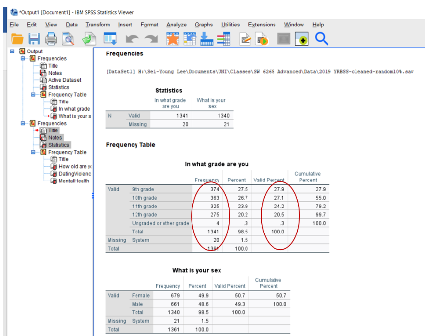
Figure 5-2. SPSS Output of Nominal and Ordinal Variables

To conduct univariate analysis for the variables of scale measures (interval and ratio levels), we tell SPSS to compute Mean, Standard Deviation, Minimum and Maximum by following the steps presented in Table 5-4 and displayed as green bubbles after red bubble steps 1 to 5 in Figure 5-1.

Figure 5-3 presents the SPSS output of univariate analysis with mean, standard deviation, minimum and maximum. We develop a table like Table 5-2 to present those values of scale variables from the SPSS Output.

Figure 5-3. SPSS Output of Scale Variables

Data Preparation 1. “Select Cases”

Using “Select Cases” depends on the research topic. Research may focus only on one specific population such as females, veterans, or older adults aged 60 or above. In case our study focuses on one gender group, then we select such cases from the dataset. The steps of selecting cases are done by following Table 5-5 and displayed in Figure 5-2. In this case selection process, the output of the case selection can be three different types: The first is to “Filter out unselected cases”, the second is to “Copy selected cases to a new dataset”, and the last is “Delete unselected cases.” The first option is to keep the original data file and filter out unselected cases. We can always remove the “filter out” option by coming back to this “Select Cases” menu and clicking “All Cases” on the first choice and “OK.” The second is to keep the original data file and create a new data file with only selected cases. Once a new data file with selected cases is created, then save the file with a new file name or the file name remains “Untitled.” The third is to delete the original data file by removing all unselected cases. We recommend the second option of creating a new SPSS data file with only selected cases.  

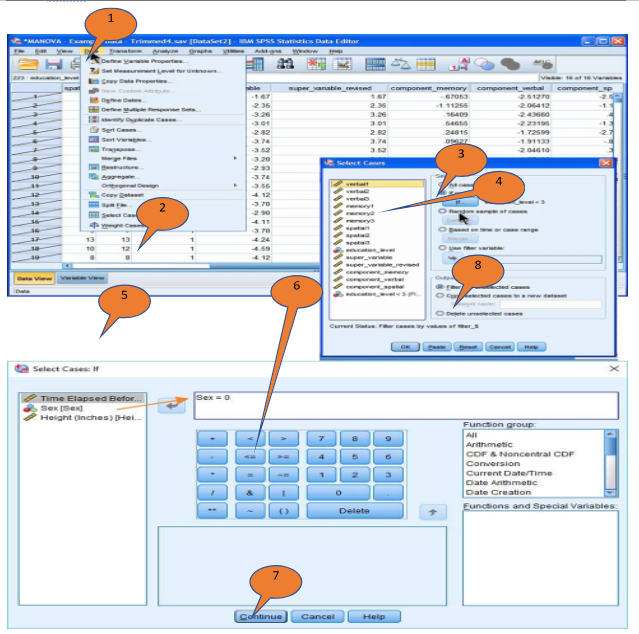
Figure 5-2. Steps to Select Cases

When we select a random sample from the dataset, we follow the same step and select “random sample of the cases” in the third option with the number of percentages we select a random sample from the original data.

Data Preparation 2. “Transform”

        “Transform” is used when we need to change the original variable to a different variable in terms of reducing the number of categories of the variable or creating a new variable from a scale-level variable to a nominal variable. When we change the variable, we can level down the original variable or reduce the number of groups of the variable. For example, we can create a new nominal or ordinal variable from a scale variable (interval or ratio measure) by collapsing the groups such as groups of 20s, 30s, 40s, and 50s from the age variable. In Table 5-1, race/ethnicity is composed of five groups; Asian, Black, Hispanic, White, and Other. We can change five groups of race/ethnicity to have two groups of White and all minorities by collapsing all minorities into one group. This transform process can be performed with “Recode” in SPSS. Figure 5-3 and Table 5-6 present steps to recode the race/ethnicity variable from five groups to two groups.

        In this “transform” process, there are two ways to do it: “Recode into Different Variable” and “Recode into Same Variable.” We recommend doing “Recode into Different Variable” to create a new variable, while keeping the original variable as is. “Recode into Same Variable” replaces existing values of the variable with new values we create. Once we recode into the same variable, the original values are overwritten and we lose old data.

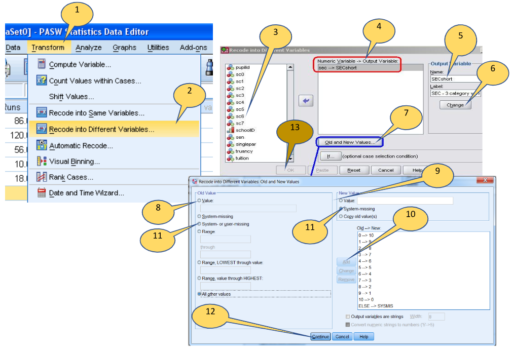
Figure 5-3. Steps to Recode a Variable

Data Preparation 3. “Compute”

        “Compute” is the function to create a new variable by calculating values like a calculator. In cases of measuring a concept with a scale such as depression with Patient Health Questionnaire - 9 (PHQ-9), Beck Depression Inventory, or self-esteem with Rosenburg Self-Esteem scale, we measure a concept with multiple scale questions and sum up the scores of all scale items to create a variable of depression or self-esteem. To create a total score of depression or self-esteem, we compute the item values, meaning adding all scale values arithmetically. Table 5-7 and Figure 5-4 Present steps to create a new variable by computing multiple values of items. With this way, we can create a new variable by subtracting and dividing the values of multiple variables.

Figure 5-4. Steps to Compute and Create a New Variable